Trimming Silence with Gaussian Mixtures

Removing silence from audio is a common task in speech machine learning applications, including wakeword/keyword detection, speech recognition, and text-to-speech. By stripping silence segments, we can reduce the amount of wasted computation used to train on a speech corpus. Doing so also enables augmentation for translation invariance, since speech segments can be padded for placement anywhere within a fixed-length context. In addition, separating speech/non-speech segments allows us to approximate the signal-to-noise (SNR) ratio of a sample and discard noisy training data.

Distinguishing silence from speech is trivial for humans, but can be a real challenge to perform automatically, especially in noisy environments. There are several algorithms that can be used for trimming silence.

Most commonly, the audio signal is normalized to a fixed reference amplitude (in dBFS), and segments of the signal below a given threshold are removed. An obvious problem with this approach is that different samples/speakers can have different dynamic ranges, so it can be difficult to determine a fixed amplitude threshold that works in all cases.

Some applications use a Voice Activity Detector (VAD) model to separate speech segments from non-speech. In my experience, VADs often behave as glorified amplitude thresholders and can be spoofed by background noise in low SNR environments. Many VAD models are designed specifically for high-recall applications like videoconferencing, so they can have a high false positive rate.

An approach I have found to be fast, accurate, and robust is to model speech/non-speech amplitudes explicitly using a Gaussian Mixture Model (GMM). GMMs require no supervised training data and are custom fit to each audio clip, so they can be used to trim silence from any sample without a global threshold.

An Example

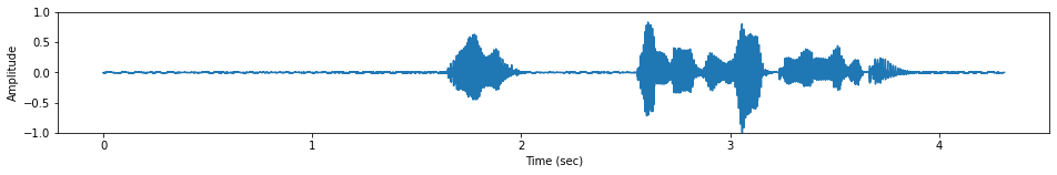
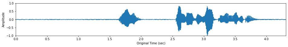
Let's take a look at an audio clip to get an idea of the problem. Below you can see that this sample has a clear excess of leading, trailing, and internal silence.

import numpy as np
import soundfile
import torch
from IPython.display import Audio, display
from matplotlib import pyplot as plt

x, fs = soundfile.read("gmm-trim/vctk1.flac")
x = torch.from_numpy(x)

Since we want to remove segments of the signal while preserving continuity (no clicks/pops), we'll first window it into overlapping frames (25ms length, 60% overlap, Hann window). We can then take the RMS of each frame as its amplitude estimate and then convert to power in dBFS.

BLOCK_LENGTH = 0.025
BLOCK_OVERLAP = 0.6

frame_length = int(BLOCK_LENGTH * fs)
frame_stride = int((1 - BLOCK_OVERLAP) * frame_length)
window = np.hanning(frame_length)

frames = x.unfold(-1, size=frame_length, step=frame_stride) * window

energy = frames.square().mean(-1).sqrt()
power = 20.0 * (energy + 1e-5).log10()

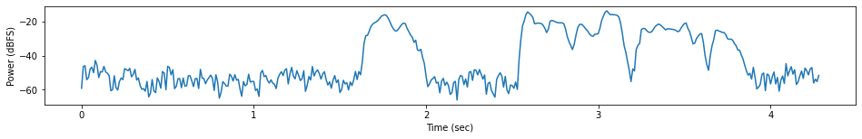
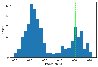
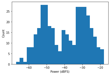
We can already see how we might go about separating the speech from silence in this clip. The histogram gives us an even better idea:

plt.xlabel("Power (dBFS)")
plt.ylabel("Count")
plt.hist(power.numpy(), bins=25)
plt.axvline(-40, color="red", linestyle="--")
plt.show()

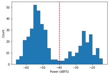
Looks like we could simply throw away any frames below -40dBFS and then reconstruct the signal from the framed representation. Of course, this approach won't generalize to all speech samples, which will vary in level, dynamic range, and SNR. But there is an automatic approach that embodies the method we used here and can generalize to virtually any speech sample.

Gaussian Mixtures

The example above makes it clear that speech amplitudes can be modeled using a bimodal distribution. We can use the Gaussian base distribution to approximate each of these modes by fitting a two-component GMM to the power vector.

A GMM is parameterized by location (mean), scale (variance), and weight vectors. For 1D data, these vectors are all length K, where K is the number of components (modes) in the mixture. The locations indicate the center position of each mode, the scales determine the width of each mode, and the weights indicate the height of each mode on the histogram.

Let's take a look at an example with some fake data. Below, we generate a dataset from two Gaussian distributions. The first has location -25, scale 100, and weight 300. The second has location -55, scale 25, and weight 700.

mode1 = 25 + np.sqrt(100) * torch.randn(300)
mode2 = 55 + np.sqrt(25) * torch.randn(700)
data = torch.cat([mode1, mode2])

plt.hist(data.numpy(), bins=30)
plt.show()

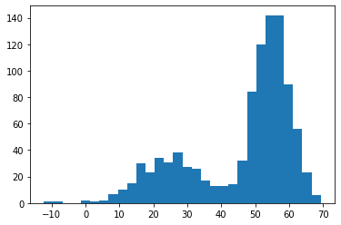
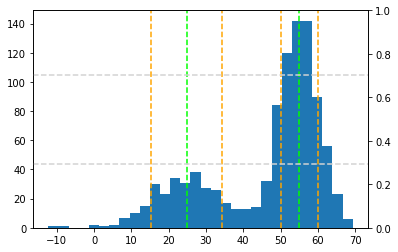
We can use sklearn to fit a GMM to this dataset using the expectation-maximization (EM) algorithm and extract the parameters from the raw data. The histogram below has been augmented with the locations in brown, locations +/- sqrt(scales) in orange, and weights in gray (separate y-axis).

import sklearn.mixture

gmm = sklearn.mixture.GaussianMixture(n_components=2).fit(data.unsqueeze(-1).numpy())

locations = gmm.means_[:, 0]
scales = gmm.covariances_[:, 0, 0]
weights = gmm.weights_

Trimming Speech

For an audio power vector, the distance between the GMM locations represents the the SNR of the signal, the scale represents the dynamic range of the corresponding signal or noise mode, and the weights indicate the relative total lengths of speech/non-speech.

We now have all the tools we need to remove the silence from an arbitrary speech sample. However, we can make the GMM fit a bit more robust by providing some initialization hints.

Normalization

By default, sklearn.mixture.GaussianMixture uses k-means clustering to find the initial location parameters from the data. This process can be slow, and we can bypass it by normalizing the audio amplitude to a fixed peak reference (-18dBFS), while preserving the dynamic range and SNR of the signal. We then recompute the energy/power of the signal.

REF_DB = -18.0

peak_energy = frames.square().mean(-1).sqrt().max()
ref_energy = 10.0 ** (REF_DB / 20.0)

gain = torch.nan_to_num(ref_energy / peak_energy)

energy = (frames * gain).square().mean(-1).sqrt()
power = 20.0 * (energy + 1e-5).log10()

Model Fitting

We can now fit a GMM to our power vector. Given our -18dB peak reference, we can choose reasonable defaults for the GMM locations at -60dB for silence and -20dB for speech. We use random initialization for the scales and weights parameters.

NOISE_INIT = -60.0
SIGNAL_INIT = -20.0

gmm = sklearn.mixture.GaussianMixture(
    n_components=2,
    init_params="random",
    means_init=np.array([NOISE_INIT, SIGNAL_INIT])[..., np.newaxis],
).fit(power.unsqueeze(-1).numpy())

modes = gmm.means_[..., 0]

noise, signal = sorted(modes)

Peak:   -18.0dB
Signal: -29.2dB
Noise:  -57.8dB
SNR:    28.6dB

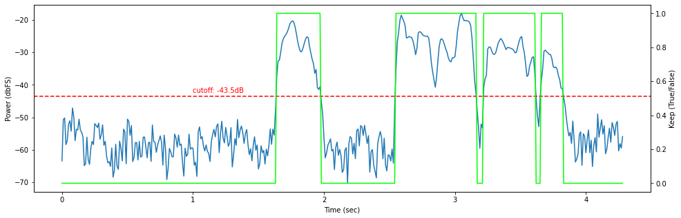
At this point, we have a model fit to our data, but we still need a way to separate speech from non-speech. I have found that simply choosing the midpoint between the two modes to be a good heuristic.

cutoff = modes.mean()
keep = power > cutoff
trimmed = frames[keep]

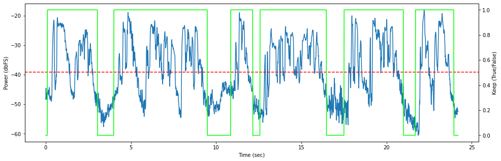
Smoothing

Right away we can see that naively discarding all frames below the threshold is noisy and loses some potentially-important frames at the edges of speech segments. Most trimming algorithms suffer from this problem, and it can be solved by applying a smoothing filter to the raw keep vector.

Below, we apply a moving average convolution over the keep values to expand the edges of speech frames by the PAD_LENGTH parameter. This parameter determines the amount of leading/trailing silence to include around each speech segment. Thus, it also determines the maximum amount of internal silence to preserve between speech segments: 2 * PAD_LENGTH.

PAD_LENGTH = 0.25

# create a moving average convolutional filter for smoothing
pad_frames = int(PAD_LENGTH * fs / frame_stride) * 2
pad_frames += 1 - pad_frames % 2
pad_weight = 1.0 / pad_frames
pad_filter = torch.full([pad_frames], pad_weight).to(keep.device)

# smooth the "keep" boolean vector
smoothed = torch.nn.functional.conv1d(
    keep.float().view(1, 1, -1),
    pad_filter.view(1, 1, -1),
    padding="same",
).flatten()

# threshold the results to keep any frames adjacent to speech
keep = smoothed >= pad_weight
trimmed = frames[keep]

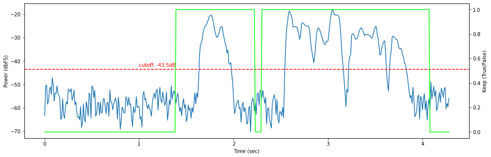
Here, we can see that the short drops in amplitude after the 3 second mark have been smoothed out, and the pause around 2 seconds has been shortened to 0.5 sec.

Resynthesis

All that remains is to re-synthesize the trimmed overlapping frames to an audio signal. This can be accomplished by a windowed overlap-and-add algorithm using PyTorch's fold function.

But first, we have to adjust the window used for analysis to be a constant-gain synthesis window. I don't want to go into the details of window function inversion, but the interested reader can find an explanation in the Griffin-Lim paper, equation 6.

# derive the synthesis window from the analysis window
overlap = -(-frame_length // frame_stride)
synth_gain = window ** 2.0
synth_gain = np.pad(synth_gain, [(0, overlap * frame_stride - frame_length)])
synth_gain = synth_gain.reshape([overlap, frame_stride])
synth_gain = synth_gain.sum(0, keepdims=True)
synth_gain = np.tile(synth_gain, [overlap, 1])
synth_gain = synth_gain.reshape([overlap * frame_stride])[:frame_length]
window /= synth_gain

# window the trimmed audio
trimmed = trimmed * torch.from_numpy(window).unsqueeze(0)

# overlap-and-add the framed results back to a flat audio signal
y = torch.nn.functional.fold(
    trimmed.transpose(0, 1).unsqueeze(0), 
    output_size=(1, (trimmed.shape[0] - 1) * frame_stride + frame_length), 
    kernel_size=(1, frame_length), 
    stride=frame_stride,
).flatten()

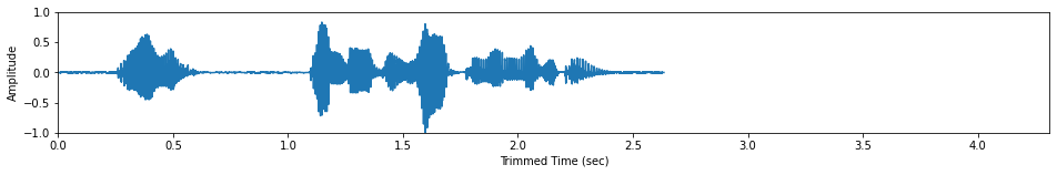
Here we can see that the algorithm removed around 1.5 sec of silence from the clip, trimming the edges and shortening the pause after "However." Note that the windowed overlap-and-add avoids any clicks or pops that could be caused by discontinuities around removed segments. The original amplitudes are also preserved by the reconstruction.

What Can Go Wrong

I have found the algorithm described above to be robust to audio examples of varying quality and dynamic range. However, it is certainly not a perfect algorithm, and here are a few pitfalls to look out for when using this approach.

Unimodality

The most common failure occurs when the signal is unimodal, which can happen if the audio contains only signal or only noise or has an extremely low SNR. Here's an example:

# generate a signal-only sine wave
x = 10 ** (REF_DB / 20) * torch.sin(2 * torch.pi * 440 * torch.arange(5 * fs) / fs)

frames = x.unfold(-1, size=frame_length, step=frame_stride) * window

energy = frames.square().mean(-1).sqrt()
power = 20.0 * (energy + 1e-5).log10()

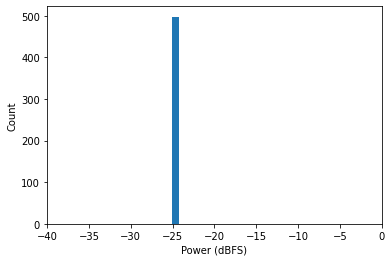
This sample is extremely unimodal, consisting of the same power level across the whole signal. When we try to fit a two-component GMM to the power vector, one of the mode's counts goes to zero, resulting in a location of zero.

gmm = sklearn.mixture.GaussianMixture(
    n_components=2,
    init_params="random",
    means_init=np.array([NOISE_INIT, SIGNAL_INIT])[..., np.newaxis],
).fit(power.unsqueeze(-1).numpy())

noise, signal = sorted(gmm.means_[..., 0])

Signal: 0.0dB
Noise:  -24.7dB
Cutoff: -12.3dB

Here, a cutoff of -12dB will be used to trim the audio signal, effectively marking all segments as silence. This can be detected in a couple of ways, and an application can choose either to keep the original signal in its entirety or discard the training example altogether.

One way to detect this case would be to apply a sanity check on the signal returned from the GMM. If it is higher than -18dB, we know that something has gone wrong, since that is our peak normalization level.

Another option would be to check the length of the trimmed output and verify that it is above a threshold. This would be a good fit for ML applications that require a minimum signal length.

Multi-Modality

The assumption that an audio sample has bimodal amplitude can be violated in some cases. Most commonly, a third mode appears for unvoiced speech. Typically, unvoiced speech falls somewhere between the amplitude modes of voiced speech and silence (usually closer to voiced speech). Here is an example:

x, fs = soundfile.read("gmm-trim/vctk2.flac")
x = torch.from_numpy(x)

frames = x.unfold(-1, size=frame_length, step=frame_stride) * window

peak_energy = frames.square().mean(-1).sqrt().max()
ref_energy = 10.0 ** (REF_DB / 20.0)

gain = torch.nan_to_num(ref_energy / peak_energy)

energy = (frames * gain).square().mean(-1).sqrt()
power = 20.0 * (energy + 1e-5).log10()

In this example, a third mode emerges for this sibilant-heavy utterance. Here's what happens when we fit the two-component GMM to the power vector.

gmm = sklearn.mixture.GaussianMixture(
    n_components=2,
    init_params="random",
    means_init=np.array([NOISE_INIT, SIGNAL_INIT])[..., np.newaxis],
).fit(power.unsqueeze(-1).numpy())

modes = gmm.means_[..., 0]
noise, signal = sorted(modes)
cutoff = modes.mean()

keep = torch.nn.functional.conv1d(
    (power > cutoff).float().view(1, 1, -1),
    pad_filter.view(1, 1, -1),
    padding="same",
).flatten() >= pad_weight

Signal: -29.7dB
Noise:  -50.8dB
Cutoff: -40.2dB

Because unvoiced consonants generally occur near voiced sounds, the smoothing filter ensures they are preserved in the trimmed audio. I found this to be true for most of the recordings I have analyzed, but it's something to keep an eye out for.

Non-Stationary Noise

In some cases, removing interior silence may introduce audible discontinuities. This is usually true for noise with a non-stationary distribution, such as music, background speech, etc. Consider this example, where we try to remove background applause from pauses in a speech with a relatively low SNR of 17dB.

x, fs = soundfile.read("gmm-trim/obama.flac")
x = torch.from_numpy(x)

Signal: -30.5dB
Noise:  -47.7dB
SNR:    17.2dB

Here the algorithm has correctly distinguished the amplified speech audio from the background crowd noise. However, trimming the noise at arbitrary points results in an audible distortion of the speech signal. Unless the background noise can be attenuated by dynamic range expansion or removed by a denoiser, this distortion is unavoidable.

Usually, the best thing to do here is to forgo attempting to remove interior silence and only trim leading/trailing silence. This can be done after filtering by taking the forward/reverse argmaxes of the keep vector:

start = keep.int().argmax()
stop = len(keep) - keep.flip(-1).int().argmax()
keep[start:stop] = True

Final Notes

Removing silence from speech recordings is a useful tool for audio ML, but it is can be nontrivial to design an algorithm that works for a wide variety of real signals. Using Gaussian Mixtures to model amplitude modes explicitly is a simple approach that has relatively few hyperparameters and no supervision.

I think it would be possible to speed up this technique a bit by training a neural network on pre-generated outputs of the GMM-based trimmer. This would avoid having to run the iterative EM algorithm for every audio clip and enable running the whole function on an accelerator (although you can also run EM on the GPU as demonstrated here).

If you are interested in a complete function implementing the technique described above, you can find one in this gist. If you have any feedback or questions, please reply here on Twitter.