Audio Bandwidth Extension with GANs

Many generative tasks in machine learning for speech synthesize audio at relatively low sample rates, usually 16kHz or 24kHz. For example, it is common for a text-to-speech pipeline to include a synthesizer that generates a mel spectrogram from text, followed by a vocoder model that outputs raw audio at 24kHz.

While these sample rates produce intelligible audio, the corresponding Nyquist frequencies (12kHz for a 24kHz sample rate) are well below the human threshold of around 20kHz. Speech clarity and timbre could therefore be improved by synthesizing speech at higher sample rates, up to the rates of the original recordings used for training.

While there have been attempts to increase the output sample rate of existing components like the vocoder, the bandwidth extension task has recently emerged as a dedicated stage of the speech pipeline. Adding a bandwidth extender after the vocoder stage enables high-fidelity synthesis without modifying the architecture of existing components or retraining them.

One such model, HiFi-GAN+, is described in the paper Bandwidth Extension is All You Need by Jiaqi Su, Yunyun Wang, Adam Finkelstein, and Zeyu Jin. The source code was not released along with the paper, so I attempted to reproduce its results in the open source library HiFi-GAN-BWE. All of my experiments are also publicly available at wandb.ai/brentspell/hifi-gan-bwe.

A Tale of Two GANs

The HiFi-GAN+ model is an update to a previous work by the same authors: HiFi-GAN, a model for denoising and dereverberation. Interestingly (and confusingly), the name was also independently used by the popular HiFi-GAN vocoder.

Indeed, since I began working on this model, a new paper has come out that attempts to unify the tasks of vocoding, bandwidth extension, and speech enhancement: HiFi++. I look forward to digging into this model and seeing how it compares with HiFi-GAN+ for bandwidth extension.

Bandwidth Extension

The task of a bandwidth extender is to reconstruct the high-frequency components of an audio signal between its Nyquist frequency (one half of the sample rate) and that of the target sample rate. For example, in order to extend an audio signal sampled at 16kHz to 48kHz, the model would need to recover frequencies in the range of 8kHz to 24kHz.

This is simultaneously an easy task and a really difficult one. Most of the audible speech signal (and certainly the most interesting bit) is well below the Nyquist cutoff, which makes the bandwidth extender a near-identity transform. This is particularly true for HiFi-GAN+, which first resamples the source signal up to the target resolution before passing it through a neural network.

On the other hand, downsampling an audio signal to a lower rate is a destructive process that usually involves a low-pass filter, which removes any sound above the Nyquist frequency. This means that the bandwidth extender must infer the high frequency components, using only the sound in the lower frequencies as input features.

HiFi-GAN+ does this without introducing noise or noticeably degrading the input signal. Let's hear some examples and see how it works. First, we'll install the library and load a pretrained model I published.

import numpy as np
import scipy.signal
import soundfile
import torch
import torchaudio
from IPython.display import Audio, Image, display
from matplotlib import pyplot as plt

torch.set_grad_enabled(False)

<torch.autograd.grad_mode.set_grad_enabled at 0x108daea60>

!pip install hifi-gan-bwe

from hifi_gan_bwe import BandwidthExtender

model = BandwidthExtender.from_pretrained("hifi-gan-bwe-10-42890e3-vctk-48kHz")

Degraded Speech

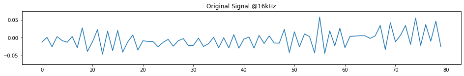
Now we can load a 48kHz audio clip and run it through the model. We'll first downsample it to 16kHz using bandlimited interpolation. Notice the audible effect of removing frequencies between 8kHz and 24kHz from the signal.

FS_DEGRADE = 16000

w, fs = soundfile.read("./hifi-gan-bwe/eldenring.wav", dtype=np.float32)
display(Audio(w, rate=fs))

x = torchaudio.functional.resample(torch.from_numpy(w), fs, FS_DEGRADE)
display(Audio(x, rate=FS_DEGRADE))

Next we'll pass the degraded signal through HiFi-GAN+ to restore it to 48kHz. Note the improved clarity and timbre of the sibilants.

y = model(x, FS_DEGRADE)

Audio(y, rate=int(model.sample_rate))

Synthetic Speech

Let's try another example, this time using synthesized speech. The following clip was generated by the Amazon Polly neural text-to-speech service. The sample was synthesized at 16kHz in the PCM format, in order to avoid any MP3 distortion in the default format.

x, fs = soundfile.read("./hifi-gan-bwe/beachmouse16kHz.wav", dtype=np.float32)

y = model(torch.from_numpy(x), fs)

display(Audio(x, rate=fs))
display(Audio(y, rate=int(model.sample_rate)))

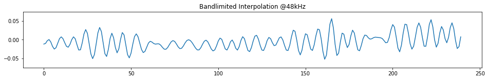
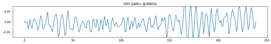
If we zoom into the signal, we can see a bit of what's going on here. Below are the raw samples from a 5ms clip of one of the sibilants. Note the over-smoothing in the simple band-limited conversion to 48kHz and the level of detail in the HiFi-GAN+ output.

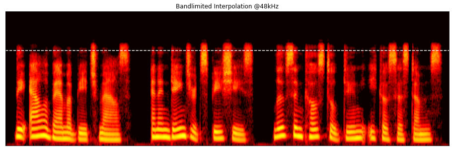
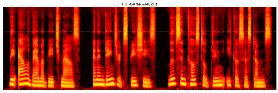
We can also see these effects in the frequency domain. Below are the log mel spectrograms for the interpolated clip and the HiFi-GAN+ outputs. Note the detail in the higher frequencies that isn't present in the original sample.

melspec_xform = torchaudio.transforms.MelSpectrogram(
    sample_rate=model.sample_rate,
    n_fft=2048,
    win_length=int(0.025 * model.sample_rate),
    hop_length=int(0.010 * model.sample_rate),
    n_mels=128,
    power=1,
)

w_spec = torch.log(melspec_xform(w) + 1e-5)
y_spec = torch.log(melspec_xform(y) + 1e-5)

Here is another example from Amazon Polly, synthesized at 8kHz and then upsampled with HiFi-GAN+:

x, fs = soundfile.read("./hifi-gan-bwe/beachmouse8kHz.wav", dtype=np.float32)
y = model(torch.from_numpy(x), fs)
display(Audio(x, rate=fs))
display(Audio(y, rate=int(model.sample_rate)))

and another, synthesized at 24kHz:

x, fs = soundfile.read("./hifi-gan-bwe/beachmouse24kHz.wav", dtype=np.float32)
y = model(torch.from_numpy(x), fs)
display(Audio(x, rate=fs))
display(Audio(y, rate=int(model.sample_rate)))

Music

Although the model was trained on speech data, it actually works pretty well with music audio. Here is an example of a song downsampled to 16kHz and then restored with HiFi-GAN+ to 48kHz.

FS_DEGRADE = 16000

x, fs = soundfile.read("./hifi-gan-bwe/rick.wav", dtype=np.float32)
display(Audio(x, rate=fs))

x = torchaudio.functional.resample(torch.from_numpy(x), fs, FS_DEGRADE)
display(Audio(x, rate=FS_DEGRADE))

y = model(x, FS_DEGRADE)
display(Audio(y, rate=int(model.sample_rate)))

Architecture

I don't want to rehash the whole paper, but I would like to highlight a few interesting points about the models used in HiFi-GAN+. The generator model consists of a stack of 16 dilated residual convolution layers inspired by the WaveNet architecture. It has a total of only 1 million parameters for lightweight inference.

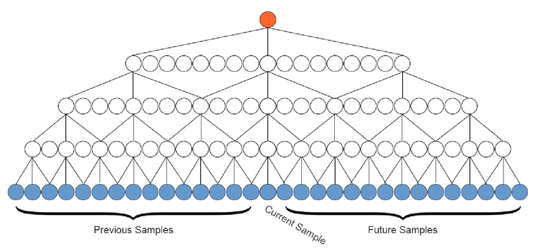
These exponential (base 3) dilations create a large receptive field, allowing long term dependencies between samples. Unlike the original WaveNet, this model uses non-causal convolutions, providing access to previous and future context when generating each sample. HiFi-GAN+ further simplifies the WaveNet model by removing the conditioning input, since the output audio signal depends only on the input signal. This allows us to implement the WaveNet layers in just a few lines of code.

As with most of these recent GAN-based raw audio models, all of the complexity is in the discriminator(s). HiFi-GAN+ uses five separate discriminator models: one 2D mel spectrogram discriminator and four 1D raw waveform discriminators, each applied to a resampled version of the input signal at varying sample rates.

Each discriminator consists of a stack of simple dense convolutions that output a linear 0/1 (fake/real) indicator for the input signal. In addition, each discriminator outputs per-layer feature maps from each convolution, which are used as an auxiliary loss term.

In addition to the standard LS-GAN losses and the feature map losses, the HiFi-GAN+ model uses several L1 reconstruction losses to train the generator. These include a raw waveform loss, four log-STFT losses at varying window sizes, and a log mel spectrogram loss, band-limited to the Nyquist frequencies between the input and target sample rates.

Training Notes

The HiFi-GAN+ paper includes excellent model/hyperparameter details, so I tried to keep the library as close to the reference as I could. Below are a few things that differ from the original experiments described in the paper.

Warmup Iterations

The authors trained their generator for 1M iterations (~100 epochs of VCTK) at a fixed learning rate of 1e-3 before training the discriminator and including adversarial losses. I found in my own experiments that training the generator to only 100K iterations (~10 epochs) results in less noise in the predicted audio. My reasoning for this is that training for longer at a high learning rate causes the model's weights to become larger, which may account for the noisier outputs.

Receptive Field Padding

The paper doesn't mention any padding or receptive field masking. However, I have found in the past that these WaveNet-style models can benefit from input or output adjustments to accommodate the large receptive field (13120 samples in HiFi-GAN+). This can be done by zero-padding the input signal on either side by half the receptive field length, or by restricting the loss calculation to samples that are fully within the receptive field (turning residual same padding into valid padding). In the HiFi-GAN-BWE library, I went with the former approach, which resulted in fewer artifacts at the edges of the audio signal due to residual convolution padding.

Sample Rate Augmentation

For their experiments, the authors train a separate model on each source sample rate (8kHz->48kHz and 16kHz->48kHz). In order to simplify the client interface and further augment the training data, I trained a single model that can upsample from an arbitrary source sample rate. During training, the library randomly selects one of 8kHz, 16kHz, or 24kHz as the source rate and downsamples the ground truth audio to that sample rate for the model's inputs.

Amplitude Augmentation

The authors use noise augmentation from the DNS Challenge dataset to reduce overfitting and improve generalization in the model. In addition to noise augmentation, I included up to 18dB of random amplitude augmentation in each training example for further generalization through amplitude independence.

Tanh Activation

It is unclear from the paper what activation is used in the final output of the HiFi-GAN+ model. While it is possible that the authors used a default linear activation, it is more likely that a nonlinearity with a range restricted to [-1, 1] was used, a common choice for raw audio ML models. Therefore, the library uses the tanh activation, which is also used by the HiFi-GAN vocoder.

Final Notes

Bandwidth extension is an interesting and useful approach for improving the signal quality of neural audio models and scaling them up to higher resolution. Of course, introducing a new stage in these pipelines increases model size, compute and memory cost, and latency.

In the case of HiFi-GAN+, the overhead is 4MB of model size and ~70MB of intermediate tensor memory usage during inference. While the model is not causal, it is possible to stream its interpolator and WaveNet convolutions, with a latency of only 15ms of forward receptive field.

While the model is fast enough for real-time streaming on the GPU, a quick test on my laptop shows that this is not the case on the CPU. From the snippet below, you can see that it has a real-time factor of barely 1/3.

%%timeit x = torch.zeros(model.sample_rate)
model(x, int(model.sample_rate))

2.74 s ± 42.5 ms per loop (mean ± std. dev. of 7 runs, 1 loop each)

I have enjoyed working through this paper and developing the open source implementation. The models are easy to reason about and train quickly on a relatively small dataset. I would love to hear any questions or feedback you have - reply on Twitter here.