Yin Pitch Estimator in PyTorch
March 19, 2022
An estimator of fundamental frequency, or pitch, of an audio signal is a useful tool for many audio machine learning applications. For example, the pitch contour is used as an input feature in the Mellotron singing synthesizer and the DDSP sound generator. Pitch vectors can also be used as a training target, as is done in the FastPitch speech synthesizer.
There are many algorithms and deep learning models for pitch estimation, but one of the most popular (even after 20 years!) is the Yin estimator by Alain de Cheveigné, et al. There is an excellent iterative implementation of this paper in NumPy by Patrice Guyot, which can produce a pitch vector for a given audio signal. However, it is possible to implement the algorithm in a vectorized, batchable, and GPU-compatible manner. To this end, I created a simple library called Torch-Yin, which implements the Yin pitch estimator in the PyTorch deep learning framework.
Pitch Estimation
Most pitch estimators assume that an audio signal is composed of periodic or aperiodic signals. To calculate the pitch, an estimator splits the whole signal into a sequence of overlapping sliding frames, each of which is analyzed independently. If the algorithm determines that a frame is periodic, it returns a fundamental frequency for it; otherwise it returns 0. The results for the whole signal are then returned as a vector of pitch values, at a spacing determined by the frame stride length.
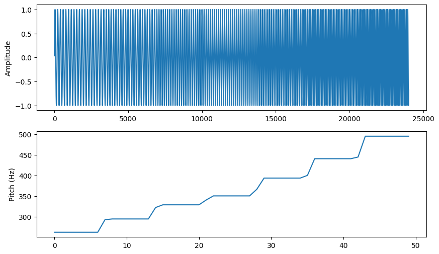
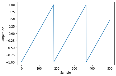
For example, the following 0.5 second audio signal at 48kHz has 24000 samples.
The corresponding pitch vector p, computed with a stride of 0.01 seconds
(100 pitches/sec) has a length of 50. For more information on how these
periodic signals are generated, see my previous post
describing oscillator synthesis.
!pip install torch-yin

import numpy as np
import soundfile
import torch
import torchyin
from IPython.display import Audio, display
from matplotlib import pyplot as plt
from tabulate import tabulate

π = np.pi
FS = 48000
PITCHES = [261.63, 293.66, 329.63, 349.23, 392.00, 440.00, 493.88]

f = np.repeat(PITCHES, FS // 2 // len(PITCHES) + 1)
y = np.sin(2 * π * (np.cumsum(f / FS) % 1.0))

p = torchyin.estimate(y, sample_rate=FS, pitch_min=200, frame_stride=0.01)

Audio(y, rate=FS)
Classical Pitch Detection
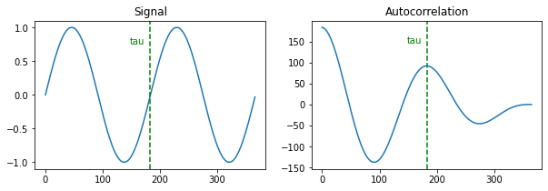
Once the signal has been framed and strided, the estimation algorithm is applied to each frame independently. At the heart of all pitch estimation algorithms is the observation that periodic signals repeat themselves after completing each cycle. This is true even for harmonic signals, which are composed of a fundamental frequency mixed with signals at integer multiples of that frequency.
$$ r_t(\tau) = \sum_{j=t+1}^{t+W}{x_j}{x_{j+\tau}} $$An efficient traditional algorithm used for determining the length of a cycle
of a periodic signal is the
autocorrelation method. Intuitively,
the autocorrelation of a signal computes the dot product of the signal with
delayed versions of itself, with each delay indicated by 𝜏 samples. This dot
product is then a measure of the similarity of the signal to the delayed
version, so the peaks of the autocorrelation correspond to the period (𝜏)
of the signal. Once the period 𝜏 is known, the frequency is just the sample
rate divided by the period (FS / 𝜏).
Here is an example of two cycles of a waveform and its autocorrelation. Note that there is a trivial peak at the start of the autocorrelation, which represents a delay of 0. If we skip this initial peak, we can compute the argmax of the rest of the signal to recover the cycle length, and thus the fundamental frequency.
FS = 48000
PITCH = 261.63
PITCH_MAX = 300
TAU_MIN = FS // PITCH_MAX

y = np.sin(2 * π * PITCH * np.arange(2 * int(FS / PITCH) + 1) / FS)
a = np.correlate(y, y, mode="full")[len(y):]
𝜏 = np.argmax(a[TAU_MIN:]) + TAU_MIN + 1

FS / 𝜏
262.2950819672131
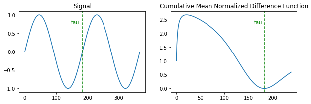
Yin Algorithm
Yin's authors describe several shortcomings of the autocorrelation method, especially when the signal amplitude is rising or falling. See the paper for details, but instead of autocorrelation, the Yin algorithm uses a squared difference function between the signal and its delayed copies. Otherwise, the steps in the algorithm are similar: window the audio into overlapping frames, compute a measure of delayed sample similarity/difference, and then search for a suitable extremum of this measure. Let's take a look at how these steps can be implemented in PyTorch.
Framing
def _frame(signal: torch.Tensor, frame_length: int, frame_stride: int) -> torch.Tensor:
    # window the signal into overlapping frames, padding to at least 1 frame
    if signal.shape[-1] < frame_length:
        signal = torch.nn.functional.pad(signal, [0, frame_length - signal.shape[-1]])
    return signal.unfold(dimension=-1, size=frame_length, step=frame_stride)
PyTorch provides the handy
unfold
function, which turns a tensor shaped [..., samples] into a tensor shaped
[..., frames, frame], allowing us to create an overlapping view of the
signal without any copying. Of course, we must first pad the signal with zeros
to the frame length, so that we get at least one frame. As an aside, it's also
important not to mutate this tensor, which would modify the underlying
audio signal in unexpected ways.
Differencing
def _diff(frames: torch.Tensor, tau_max: int) -> torch.Tensor:
    # compute the frame-wise autocorrelation using the FFT
    fft_size = 2 ** (-int(-np.log(frames.shape[-1]) // np.log(2)) + 1)
    fft = torch.fft.rfft(frames, fft_size, dim=-1)
    corr = torch.fft.irfft(fft * fft.conj())[..., :tau_max]

    # difference function (equation 7)
    sqrcs = torch.nn.functional.pad((frames * frames).cumsum(-1), [1, 0])
    corr_0 = sqrcs[..., -1:]
    corr_tau = sqrcs.flip(-1)[..., :tau_max] - sqrcs[..., :tau_max]
    diff = corr_0 + corr_tau - 2 * corr

    # cumulative mean normalized difference function (equation 8)
    return (
        diff[..., 1:]
        * torch.arange(1, diff.shape[-1])
        / np.maximum(diff[..., 1:].cumsum(-1), 1e-5)
    )
This is the heart of the Yin algorithm, and the most confusing/handwavy part, as described in section II.B and II.C of the paper. Surprisingly, while the algorithm is based on a completely new difference function (equation 7), it actually uses the autocorrelation calculation to compute the result!
It also turns out that it can be much more efficient (for large frames) to
compute the autocorrelation using the Fast Fourier Transform (FFT), as
described by the
Wiener–Khinchin theorem.
This is an important optimization in Guyot's
implementation
that we use as a reference. The first block of the _diff function above
performs an optimally-sized FFT on the framed signal, multiplies the result
by its conjugate, and then computes the inverse FFT to return to the sample
domain. Note that PyTorch's
conv1d
op computes the correlation (and thus could be used for autocorrelation), but
it doesn't support batch dimensions on the second parameter, so we use the
FFT method instead.
Another contribution/optimization made in the reference implementation is to
compute the two "energy" terms corr_0 (${r_t(0)}$) and corr_tau
(${r_{t + \tau}(0)}$) using a single cumulative sum over the delay-0
autocorrelation. I think this technique was discovered by simplifying and
canceling terms in equations 1 and 7, but we'll leave the full derivation as
an exercise for the reader.
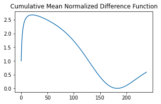
Finally, we compute the cumulative mean normalized difference function (CMDF) directly from equation 8 in the paper. Compare the CMDF below to the autocorrelation calculated earlier. The minima of the CMDF values are used to find the fundamental period 𝜏 in the search algorithm.
FS = 48000
PITCH = 261.63
PITCH_MIN = 200
TAU_MAX = FS // PITCH_MIN

y = np.sin(2 * π * PITCH * np.arange(2 * int(FS / PITCH) + 1) / FS)
cmdf = _diff(torch.from_numpy(y), tau_max=TAU_MAX)
Searching
In order to find the desired minimum of the CMDF, Guyot's implementation performs a linear search, ignoring periods outside the minimum/maximum pitch range and applying a threshold filter, ignoring any CMDF values above the threshold.
We want our PyTorch implementation to be able to run on the GPU and support batching, so we can't use this simple iterative search. Fortunately, there is a straightforward way to find the index of the first matching value in a tensor without iterating, the argmax function!
To do this, we rely on the documented behavior that the argmax function returns the first index of the maximum value if there are multiple occurrences. Doing this for a tensor of Boolean values allows us to perform a vectorized linear search using an arbitrary criteria. Unfortunately, PyTorch doesn't currently support the argmax function on Boolean tensors directly, but we can easily convert it to a 0/1 integer tensor first. For example, we can find the index of the first even number in the following tensor:
x = torch.tensor([3, 1, 4, 1, 5, 9, 2, 6, 5, 3, 5, 8, 9, 7, 9, 3])
b = x % 2 == 0
b.int().argmax()
tensor(2)
b = x == 0
b.int().argmax()
tensor(0)
Note in the second example that if no match is found, argmax returns 0, since all values are False. With this trick in place, we are now ready to search for 𝜏.
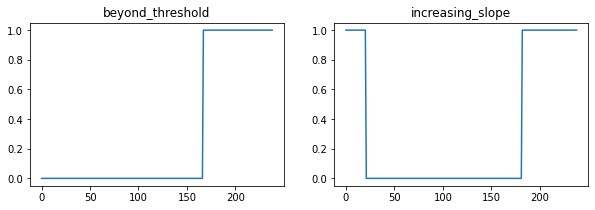
def _search(cmdf: torch.Tensor, tau_max: int, threshold: float) -> torch.Tensor:
    # mask all periods after the first cmdf below the threshold
    # if none are below threshold (argmax=0), this is a non-periodic frame
    first_below = (cmdf < threshold).int().argmax(-1, keepdim=True)
    first_below = torch.where(first_below > 0, first_below, tau_max)
    beyond_threshold = torch.arange(cmdf.shape[-1]) >= first_below

    # mask all periods with upward sloping cmdf to find the local minimum
    increasing_slope = torch.nn.functional.pad(cmdf.diff() >= 0.0, [0, 1], value=1)

    # find the first period satisfying both constraints
    return (beyond_threshold & increasing_slope).int().argmax(-1)
Guyot's search has a compound condition that 𝜏 must be
beyond the
index of the first CMDF value below the harmonic threshold parameter,
and that the CMDF must be
sloping upward.
That is, the algorithm finds the local minima of CMDF values below the
threshold. This means that we can conjoin the two conditions into a single
Boolean tensor and use the argmax to find 𝜏. The threshold also tells us
whether the signal is periodic at all, since we return 0 for 𝜏 if no CMDF
values are below the threshold.
Once the fundamental period 𝜏 has been found (or is 0 for an aperiodic signal), we can easily convert it to a fundamental frequency and return.
Performance
On my laptop CPU, the TorchYin implementation runs with default parameters and a 44.1kHz sample rate for a 1 second audio sample at the following speed.
%%timeit FS = 44100; y = np.sin(2 * π * 261.63 * np.arange(FS) / FS)
torchyin.estimate(y, FS)
26.8 ms ± 563 µs per loop (mean ± std. dev. of 7 runs, 10 loops each)
However, especially on the CPU, performance is heavily dependent on the
algorithm's configuration. In particular, the pitch_min parameter determines
the length of the sliding windows (smaller pitch_min values mean larger
windows), and frame_stride determines the number of windows that must be
processed for a given audio sample. The audio sample_rate also affects
running time, but is not usually adjusted for performance purposes. And of
course, adding more signals to a batch will increase the running time.
For example, the following configuration is typical for a speech processing application.
%%timeit FS = 16000; y = np.sin(2 * π * 261.63 * np.arange(FS) / FS)
torchyin.estimate(y, FS, pitch_min=100, pitch_max=500)
1.03 ms ± 46.7 µs per loop (mean ± std. dev. of 7 runs, 1,000 loops each)
The situation is a bit more complicated on the GPU, since we have much more granular parallelism to work with. However, once the available parallelism has been saturated, performance will degrade as on the CPU. As with all deep learning workloads, the pitch estimator must be profiled and tuned specifically for the accelerator and task at hand.
Some Examples
Aperiodic Signals
For non-periodic signals, the pitch estimator should return 0. In the examples below, we can see that silence and Gaussian/uniform noise are correctly detected as aperiodic.
FS = 48000

y = np.vstack([
    np.zeros(FS),
    np.random.normal(size=FS),
    np.random.uniform(-1, 1, size=FS),
])

torchyin.estimate(y, sample_rate=FS)[:, 0]
tensor([0., 0., 0.], dtype=torch.float64)
Harmonic Signals
Harmonic signals are an additive mix of a fundamental frequency (F0) and integer multiples of that frequency, with decreasing amplitude for higher order harmonics. The pitch detector should return the frequency of the fundamental for these signals. For example, the sawtooth wave at 261.63Hz below has harmonics at all integer frequencies (261.63, 523.26, 784.89, etc).
FS = 48000

y = 2 * (np.cumsum(np.full(FS, 261.63) / FS) % 1.0) - 1
torchyin.estimate(y, sample_rate=FS)[0].item()
262.2950819672131
Music Notes
In this example, we generate signals for each of the 88 standard piano keys at a 400Hz tuning. Note that we use a much higher sample rate for these signals, which improves the accuracy of the pitch estimator for higher fundamental frequencies. The log-scale plot shows the predicted pitch values and the absolute pitch error, which increases roughly linearly with the pitch.
FS = 96000
FREQS = 2 ** ((np.arange(88) - 48) / 12) * 440

t = np.arange(FS) / FS
y = np.vstack([np.sin(2 * π  * f * t) for f in FREQS])
p = torchyin.estimate(y, sample_rate=FS)[:, 0].numpy()

# broadcast the absolute errors into a matrix for all notes
errors = np.abs(p[np.newaxis, :] - FREQS[:, np.newaxis])
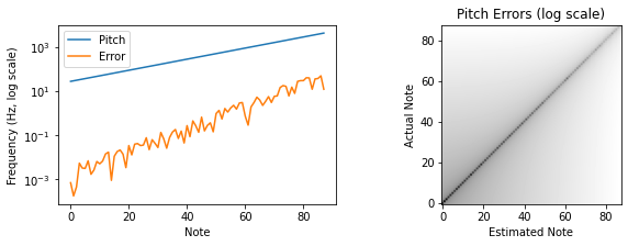
We can also verify that the note frequency nearest to each predicted pitch matches the expected note (this check was taken directly from the Torch-Yin unit tests). Here we use the indexes of the note list and compare the argmin of the absolute error matrix to ensure that the indexes line up correctly.
expect = np.arange(len(FREQS))
actual = np.argmin(errors, axis=-1)
(expect == actual).all()
True
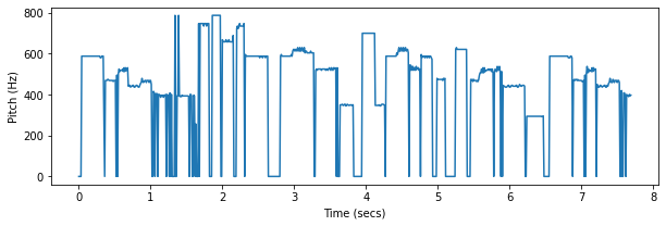
Music
Here we apply the algorithm to a much more challenging task: detecting the pitch of a monophonic piano recording. You can see where the pitch detector struggles with the rapid note changes and the long release time of the piano.
y, fs = soundfile.read("./pytorch-yin/fugue-in-g-minor.flac", always_2d=True)
y = y.sum(-1)

p = torchyin.estimate(y, sample_rate=fs, pitch_min=200, pitch_max=1000)

Audio(y, rate=fs)
We can also listen to the algorithm by stretching the pitch detector's outputs to the audio sample rate and then synthesizing a signal corresponding to each detected pitch. This is a nice way to debug the implementation or tune its configuration parameters.
f = np.repeat(p, -(-len(y) // len(p)))
y_p = np.sin(2 * π * (np.cumsum(f / fs) % 1.0))[:len(y)]

Audio(y_p, rate=fs)
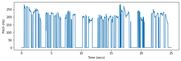
Speech
Finally, one of the most common uses of pitch detection is for speech, with applications in speaker detection, text-to-speech, voice conversion, and many other tasks. Note that, compared to music, the pitch range of ordinary speech is usually much narrower.
y, fs = soundfile.read("./pytorch-yin/firekeeper.flac", always_2d=True)
y = y.sum(-1)

p = torchyin.estimate(y, sample_rate=FS, pitch_min=100, pitch_max=300).numpy()

Audio(y, rate=fs)
We can again synthesize a sinusoid that corresponds to the detected pitch contour. Here we also mix the synthesized sample with the original audio so you can hear the pitch errors.
f = np.repeat(p, -(-len(y) // len(p)))
y_p = np.sin(2 * π * (np.cumsum(f / fs) % 1.0))[:len(y)]
y_mix = 0.5 * y_p + y

display(Audio(y_p, rate=fs))
display(Audio(y_mix, rate=fs))
Over a large collection of recordings, vocal features can be extracted from raw pitch contours and associated with the speaker for downstream tasks. Below are the speaker's mean F0 and 90th percentile range for this recording.
voiced = p[p > 0]
mean = voiced.mean()
min_, max_ = np.percentile(voiced, [5, 95])

print(f"Mean Pitch:  {mean:0.0f}Hz")
print(f"Vocal Range: {min_:0.0f}Hz - {max_:0.0f}Hz")
Mean Pitch:  213Hz
Vocal Range: 175Hz - 257Hz
Final Notes
The Yin pitch detector is fast and accurate for monophonic audio, and the Torch-Yin library provides an easy way to integrate the algorithm into a PyTorch deep learning pipeline. For multi-source signals, a source separation algorithm such as Demucs can be applied, and then the pitch detector run on each source. Polyphonic pitch detection, along with Automatic Music Transcription (AMT), are active research areas with new papers coming out regularly.
As always, if you have any feedback or questions, please reply here.