Efficient Oscillator Synthesis

Oscillators are basic building blocks for several sound generation algorithms, such as additive, subtractive, and frequency modulation (FM) synthesis. For digital synthesizers, these waveforms are represented by points sampled from a continuous periodic function. In most cases, we can generate these samples efficiently in Python/NumPy in a vectorized manner, instead of one sample at a time.

import matplotlib as mpl
import numba
import numpy as np
from IPython.display import Audio, display
from matplotlib import pyplot as plt

π = np.pi

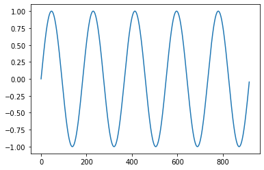
Let's start with a simple constant frequency sinusoid:

FS = 48000      # audio sample rate, in Hz
DURATION = 1.0  # sample duration, in seconds
FREQ = 261.63   # sound frequency, in Hz (middle C)

t = np.arange(int(DURATION * FS))
y = np.sin(2 * π * FREQ / FS * t)

Here, we use the fact that the closed form equation for a sinusoid is

where A is the amplitude, f is the (rate-normalized) frequency, t is the index of each sample, and ${\phi}_0$ is the phase offset (0 usually). This allows us to generate all samples for the oscillator at once.

Varying Frequency

Let's try an example with a modulated frequency using a 2Hz Low-Frequency Oscillator (LFO).

lfo = np.sin(2 * π * 2 / FS * t)
f = FREQ + 100 * lfo
y = np.sin(2 * π * f / FS * t)

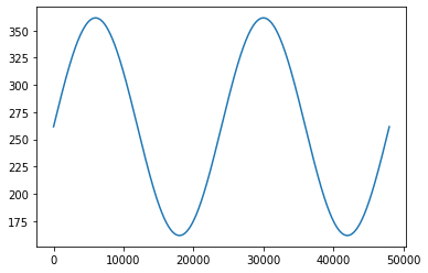
The plot above shows the expected frequency of the sound over time, as modulated by the LFO. This is clearly not what the audio sounds like. What went wrong? It turns out that the equation above is not quite correct for a variable frequency sinusoid. The more general sinusoid equation is

Here, ${\phi}(t)$ is the instantaneous phase of the oscillator. In the incorrect example above, we were using $f(t){\cdot}t$ to generate the sinusoid, where $f(t)$ is the instantaneous frequency.

The instantaneous phase is the integral of the instantaneous frequency. This means that, for a time-varying frequency, we have to integrate (sum) all the instantaneous frequencies to generate the correct phase and waveform. Using the same LFO and frequency vector from above, the correct signal can be generated as follows.

p = np.cumsum(f / FS)
y = np.sin(2 * π * p)

Note that for constant frequency waveforms, we were able to get by using $f{\cdot}t$ as the instantaneous phase, because

Phase Wrapping

Let's check that this version still works for the constant frequency case. For the purposes of comparison, we throw away the first sample in the original, since np.cumsum doesn't start at 0.

y0 = np.sin(2 * π * FREQ / FS * np.arange(10 * FS))[1:]
y1 = np.sin(2 * π * np.cumsum(np.full(10 * FS, FREQ / FS)))[:-1]

np.allclose(y0, y1)

False

What's going on here? The clips sound the same, but there is a subtle mismatch between the two waveforms. Here's a plot of the L1 difference:

plt.plot(np.abs(y0 - y1))

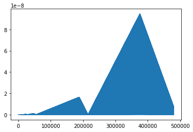
This difference is caused by roundoff error in y1 as the cumulative sum grows over time and loses fractional precision. To fix this, we can take advantage of the fact that oscillators are periodic functions that "wrap around" when they exceed their period. Unfortunately, NumPy doesn't have a modular version of its cumsum function, but we can build an efficient version of it using Numba.

@numba.jit
def modcumsum(x, m):
    y = np.empty_like(x)
    y[0] = x[0]
    for i in range(1, len(x)):
        y[i] = (y[i - 1] + x[i]) % m
    return y

The modcumsum function will compute a cumulative sum of the values in x modulo m. Numba JIT-compiles this function to LLVM, which gives us native performance for the iterative algorithm. We can now generate a numerically stable sinusoid oscillator by accumulating phases modulo 1.

y0 = np.sin(2 * π * FREQ / FS * np.arange(10 * FS))[1:]
y1 = np.sin(2 * π * modcumsum(np.full(10 * FS, FREQ / FS), 1))[:-1]

np.allclose(y0, y1)

True

Just for fun, let's see how much faster the compiled version runs than the original Python implementation for a 10 second audio clip.

%%timeit y = np.zeros(10 * FS)

py_modcumsum = modcumsum.py_func
py_modcumsum(y, 1)

208 ms ± 6.2 ms per loop (mean ± std. dev. of 7 runs, 1 loop each)

%%timeit y = np.zeros(10 * FS)

modcumsum(y, 1)

2.11 ms ± 96.3 µs per loop (mean ± std. dev. of 7 runs, 100 loops each)

Alternatively, we can use the built-in wrapping semantics for unsigned integers to implement phase accumulation. This allows us to use np.cumsum directly without any Numba support, although it is slightly slower because it creates temporary arrays for the intermediate calculations.

def np_modcumsum(x, m):
    uint64_max = 2**64 - 1
    return np.cumsum(x / m * uint64_max, dtype=np.uint64) / uint64_max * m

%%timeit y = np.zeros(10 * FS)

np_modcumsum(y, 1)

2.46 ms ± 139 µs per loop (mean ± std. dev. of 7 runs, 100 loops each)

Other Oscillators

The sine wave is pretty boring from a synthesis perspective, because it doesn't contain any harmonics beyond the fundamental frequency. However, we can use the same phase accumulation technique to implement other interesting oscillators. We'll use the pre-computed phase p below, which represents a linear-swept frequency from 100Hz to 200Hz, in the following examples.

p = modcumsum(np.linspace(100, 200, int(DURATION * FS)) / FS, 1)

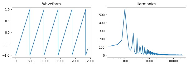
Sawtooth

Arguably the most useful primitive oscillator is the sawtooth, which generates all harmonics, each of which has an amplitude inversely proportional to its harmonic number. Once we have a correct phase accumulator, the sawtooth computation is simple - we just need to shift and scale it to [-1, 1].

def sawtooth(x):
    return 2 * x - 1

y = sawtooth(p)

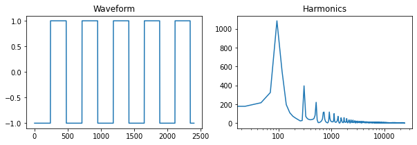
Square/Pulse Wave

The square wave has odd harmonics with the same amplitude as those of the sawtooth, and it can be generated by taking the sign of a sawtooth wave.

def square(x):
    return np.sign(sawtooth(x))

y = square(p)

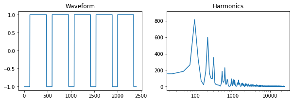
A variant of the square wave is the pulse wave, which has a duty cycle other than 0.5. Here is an example with a 75% duty cycle.

def pulse(x, duty):
    return np.sign(p / (1 - duty) - 1)

y = pulse(p, duty=0.75)

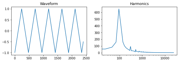
Triangle Wave

The triangle wave can also be derived from the square wave and has odd harmonics that fall off proportionally to $1/h^2$, where h is the harmonic number.

def triangle(x):
    return 1 - 2 * np.abs(sawtooth(p))

y = triangle(p)

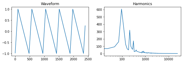
Just like the square wave, the triangle wave has an asymmetric variant, which skews the peak of the wave away from the center. Here's an example:

def triangle(x, center=0.5):
    y1 = np.clip((1 / center) * x, 0, 1)
    y2 = np.clip(1 / (1 - center) - (1 / (1 - center)) * x, 0, 1)
    return 2 * y1 * y2 - 1

y = triangle(p, center=0.2)

Better Vectorization

Some of these unit generators create several intermediate NumPy arrays in order to return the final result (the asymmetric triangle generates 6). We can use Numba again to vectorize the oscillator calculation and avoid these temporary arrays. This is done by reimplementing the oscillator in terms of individual scalar samples, and then using numba.vectorize to compile it to a NumPy ufunc. Note that the only changes we need to make are to add the Numba decorator and remove the calls to np.clip.

@numba.jit
def nb_clip(x, a, b):
    return max(a, min(x, b))

@numba.vectorize
def nb_triangle(x, center):
    y1 = nb_clip((1 / center) * x, 0, 1)
    y2 = nb_clip(1 / (1 - center) - (1 / (1 - center)) * x, 0, 1)
    return 2 * y1 * y2 - 1

y = nb_triangle(p, 0.2)

Here, we see a modest 3x gain in execution time, but we also benefit from reduced memory/GC pressure and better cache utilization, because the oscillator doens't have to create copies of the signal vector for each intermediate calculation. These improvements can be significant for long audio clips.

%%timeit x = np.zeros(10 * FS)

triangle(x, 0.75)

3.68 ms ± 232 µs per loop (mean ± std. dev. of 7 runs, 100 loops each)

%%timeit x = np.zeros(10 * FS)

nb_triangle(x, 0.75)

1.09 ms ± 51.2 µs per loop (mean ± std. dev. of 7 runs, 1,000 loops each)

Lookup Tables

When implementing an oscillator, we aren't limited to closed form functions. It is also possible to use phase accumulation to index into any single-cycle waveform represented as a vector of samples. This technique is called lookup table (LUT) synthesis and is the basis of wavetable synthesis.

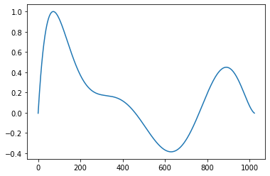
In this example, we'll fit a 7th degree polynomial to a set of random data points, evaluate that polynomial to generate a fixed-length waveform, and then use linear interpolation to synthesize an audio clip at a desired fundamental frequency. For continuity purposes, we artificially add control points at the beginning and end at $y=0$.

L = 1024
P = 10

# generate random polynomial control points
x = np.linspace(0, L, P)
y = np.hstack([0, np.random.normal(size=P - 2), 0])

# fit the random polynomial
p = np.polyfit(x, y, deg=7)

# generate and normalize the single cycle waveform to use for synthesis
w = np.polyval(p, np.arange(L))
w /= np.max(np.abs(w))

plt.plot(w)

Now that we have our base waveform, we can use our trusty phase accumulator and linear interpolation to warp it to the desired audio frequencies. Here we'll use an exponentially rising frequency from 500Hz to 4kHz.

base = 1000
f = (base**np.linspace(0, 1, int(0.3 * FS)) - 1) / (base - 1) * 3500 + 500

z = np.linspace(0, 1, len(w))
p = modcumsum(f / FS, 1)
y = np.interp(p, z, w)

Audio(y, rate=FS)

In the above example, f is our time-varying frequency, z is a linear interpolation domain over the samples in the base waveform, and p is the usual phase accumulator over f.

Wavetable synthesis extends LUT synthesis by using multiple source waveforms. The base waveforms are all the same length (usually a power of 2 samples - 256, 2048 are common) and stored consecutively in a WAV file. An additional accumulator/oscillator is used to index into the wavetable, which selects the waveform(s) to use for synthesizing each sample.

This index can even be used to interpolate between the nearest pair of waveforms. So wavetable synthesis can be thought of as a two-dimensional interpolator, where one phase accumulator is used to interpolate across the waveforms in the table, and another is used to interpolate the samples in the waveform, which produces the final signal. WaveEdit is a free tool that shows this technique in action and lets you design custom wavetables.

Final Notes

The unit generators described above are all pretty boring. More interesting sounds can be made by modulating, enveloping, filtering, mixing, and adding noise to these primitive sounds. The higher-level operations can even be driven by their own oscillators: the cutoff for a low-pass filter can be swept by its own LFO, for example.

Through vectorization and native compilation, even a slow language like Python can be used for sound generation. These efficient unit generators can even be driven by a MIDI controller using Mido and played to PyAudio in real time.

Of course, not all sound synthesis algorithms support efficient vectorization and parallelization. For example, Infinite Impulse Response (IIR) filters and other effects/modulators that use feedback must be computed one sample at a time. However, JIT compilation can still be used to reach native speeds for these iterative algorithms.

Please reply with any feedback or comments you have here.