Piecewise Interpolation in TensorFlow
January 29, 2022
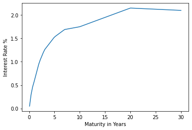
NumPy's interp
is a handy function for generating an array from a piecewise linear
mapping defined by a set of control points. For example, here is a linear plot
of today's U.S. Treasury yield curve:
import typing

import hypothesis
import numpy as np
import scipy.signal
import tensorflow as tf
from hypothesis.extra import numpy as hypnum
from IPython.display import Audio, display
from matplotlib import pyplot as plt
from tabulate import tabulate

π = np.pi
xs = [1, 2, 3, 6, 12, 24, 36, 60, 84, 120, 240, 360]
ys = [0.05, 0.09, 0.19, 0.39, 0.58, 0.99, 1.25, 1.53, 1.69, 1.75, 2.15, 2.10]
x = np.linspace(min(xs), max(xs), 100)
y = np.interp(x, xs, ys)
This function can be useful in ML applications for thresholding ROC curves,
decaying learning rates, and performing other linear calculations.
Unfortunately, there is currently no vectorized implementation of
np.interp in TensorFlow or PyTorch, but it is straightforward to implement
a piecewise interpolator using existing primitives.
Vectorized Interpolation
For eager-mode TensorFlow/PyTorch applications, it is easy enough to call
np.interp directly, and NumPy will do the right thing with tensor inputs.
However, these calls cannot be made in graph contexts, such as tf.function
or TorchScript. It is also possible to use tf.numpy_function to wrap
np.interp, but doing so limits parallelism, since the TensorFlow runtime
must call back into Python.
Instead, the following function can be used as a fully-vectorized analog of
np.interp for TensorFlow that is compatible with graph mode.
def tf_interp(x: typing.Any, xs: typing.Any, ys: typing.Any) -> tf.Tensor:
    # determine the output data type
    ys = tf.convert_to_tensor(ys)
    dtype = ys.dtype

    # normalize data types
    ys = tf.cast(ys, tf.float64)
    xs = tf.cast(xs, tf.float64)
    x = tf.cast(x, tf.float64)

    # pad control points for extrapolation
    xs = tf.concat([[xs.dtype.min], xs, [xs.dtype.max]], axis=0)
    ys = tf.concat([ys[:1], ys, ys[-1:]], axis=0)

    # compute slopes, pad at the edges to flatten
    ms = (ys[1:] - ys[:-1]) / (xs[1:] - xs[:-1])
    ms = tf.pad(ms[:-1], [(1, 1)])

    # solve for intercepts
    bs = ys - ms*xs

    # search for the line parameters at each input data point
    # create a grid of the inputs and piece breakpoints for thresholding
    # rely on argmax stopping on the first true when there are duplicates,
    # which gives us an index into the parameter vectors
    i = tf.math.argmax(xs[..., tf.newaxis, :] > x[..., tf.newaxis], axis=-1)
    m = tf.gather(ms, i, axis=-1)
    b = tf.gather(bs, i, axis=-1)

    # apply the linear mapping at each input data point
    y = m*x + b
    return tf.cast(tf.reshape(y, tf.shape(x)), dtype)
This function first converts all inputs to float64 (like NumPy), and then
pads the control points to cover the whole domain of the mapping. The
slope/intercept values of the linear parts are then solved directly, using the
familiar y = mx + b equation.
At this point, the implementation diverges from the NumPy version. For each
input x, NumPy locates the corresponding line equation using a binary
search. In the vectorized implementation, we construct the full grid of
[xs, x] values and locate the index of the first value in xs that is
greater than the input x using the argmax function. After that, we simply
apply the linear equation at that index to compute the result.
To see how this works, consider a lookup of the x vector [5, 65] in the
treasury yield example from above. The xs[..., tf.newaxis, :] > x[..., tf.newaxis]
comparison broadcasts the vectors into the following Boolean matrix:
| 1 | 2 | 3 | 6 | 12 | 24 | 36 | 60 | 84 | 120 | 240 | 360 | |
|---|---|---|---|---|---|---|---|---|---|---|---|---|
| 5 | 0 | 0 | 0 | 1 | 1 | 1 | 1 | 1 | 1 | 1 | 1 | 1 |
| 65 | 0 | 0 | 0 | 0 | 0 | 0 | 0 | 0 | 1 | 1 | 1 | 1 |
The argmax function has a convention to return the index of the first match
if the maximum value is duplicated in the array, which results in an index of
3 for an input of 5 and 8 for 65. These indexes are then used to select the
appropriate linear parameters for interpolation.
The tradeoff in this approach is that it creates a tensor containing size(x) * size(xs)
elements to perform the lookup, instead of using NumPy's CPU-parallel binary
search. This intermediate tensor can become large if there are a lot of
points to interpolate or control points. However, the lookup is performed in
effectively constant time on a GPU, which can be much faster than NumPy when
there are a lot of points to interpolate.
Testing
How do we know it works? Since we have a baseline implementation in NumPy, we can simply compute our outputs for the same inputs and compare. The Hypothesis property testing framework lets us do this without hard-coding any example arrays.
@hypothesis.given(
    x=hypnum.arrays(
        dtype=hypnum.floating_dtypes(),
        shape=hypnum.array_shapes(),
        elements=dict(min_value=-1, max_value=1)
    ),
    xs=hypnum.arrays(
        dtype=hypnum.floating_dtypes(),
        shape=hypnum.array_shapes(max_dims=1),
        unique=True,
        elements=dict(min_value=-1, max_value=1)
    ),
    ys=hypnum.arrays(
        dtype=hypnum.floating_dtypes(),
        shape=hypnum.array_shapes(max_dims=1),
        elements=dict(min_value=-1, max_value=1)
    ),
)
def test_interp(x, xs, ys):
    xs, ys = xs[:len(ys)], ys[:len(xs)]
    xs = np.sort(xs)

    expect = np.interp(x, xs, ys).astype(ys.dtype)
    actual = tf_interp(x, xs, ys).numpy()
    assert np.allclose(expect, actual), f"expect={expect} actual={actual}"

test_interp()
The test first sorts the interpolation domain (xs) and ensures it contains
unique values, which is an assumption made by all of these interp functions.
We also restrict the ranges of all values to [-1, 1], in order to avoid
rounding/overflow inconsistencies between the frameworks.
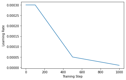
Application: Piecewise Learning Rate Schedule
As an example, we'll implement a piecewise linear learning rate decay
for TensorFlow. This learning rate scheduler can be used with any tf.keras
optimizer. It is configured with a sorted list of training steps and
corresponding learning rates. The learning rate returned to the optimizer will
be interpolated based on this schedule.
class PiecewiseLinearSchedule(tf.keras.optimizers.schedules.LearningRateSchedule):
    def __init__(self, steps: typing.List[int], rates: typing.List[int]):
        if steps != sorted(steps):
            raise ValueError("steps should be listed in ascending order")

        self._steps = steps
        self._rates = rates

    def __call__(self, step: tf.Tensor) -> tf.Tensor:
        return tf_interp(step, self._steps, self._rates)

learning_rate = PiecewiseLinearSchedule([100, 500, 1000], [3e-4, 5e-5, 1e-5])
For an example usage, we'll train a simple DNN logistic regression model on
the XOR function, a classic "Hello World" problem for neural networks. Note
that the training step function train uses the tf.function decorator for
graph mode training, which allows us to take advantage of the tf_interp
function we implemented above.
model = tf.keras.Sequential(
    [
        tf.keras.layers.Dense(units=256, activation="relu"),
        tf.keras.layers.Dense(units=1)
    ]
)
criterion = tf.keras.losses.BinaryCrossentropy(from_logits=True)
optimizer = tf.keras.optimizers.Adam(learning_rate=learning_rate)


@tf.function
def train(inputs: tf.Tensor, targets: tf.Tensor) -> None:
    with tf.GradientTape() as tape:
        outputs = model(inputs, training=True)
        loss = criterion(targets, outputs)

    optimizer.minimize(loss, model.trainable_variables, tape=tape)


# fit on random batches of binary inputs and XOR targets
for _ in range(1000):
    x = tf.random.uniform([32, 2]) < 0.5
    y = x[:, :1] ^ x[:, 1:]
    train(x, y)
We can then evaluate the trained model on the truth table to verify it has learned XOR.
x = np.array([[0, 0], [0, 1], [1, 0], [1, 1]])
y = tf.nn.sigmoid(model(x)).numpy()[..., 0]

for (a, b), c in zip(x, y):
    print(f"{a:^} ⊕ {b:^} = {c > 0.5:^}")
0 ⊕ 0 = 0
0 ⊕ 1 = 1
1 ⊕ 0 = 1
1 ⊕ 1 = 0
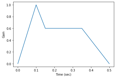
Application: ADSR Envelope Generator
Piecewise linear functions are also commonly used to model ADSR envelopes for music synthesis. For example, an envelope can be used to control the timbre of an instrument as keys are pressed, held, and released, by shaping the amplitude of the audio signal.
The attack, decay, and release parameters specify the amount of
time for the envelope to transition between stages, corresponding to the
xs parameter in the interpolator. The sustain parameter indicates
the gain that the envelope should decay to and hold while the instrument's
key remains pressed.
The envelope generator below demonstrates how the ADSR parameters correspond to piecewise interpolator control points. The envelope begins at 0 gain, rises through the attack stage to full gain, decays to the sustain level, and then decays back to 0 in the release stage. All time values are represented in seconds.
def adsr(attack, decay, sustain, release):
    def gen(time):
        hold = max(time[-1] - (attack + decay + release), 0)
        xs = np.cumsum([0, attack, decay, hold, release])
        ys = [0, 1, sustain, sustain, 0]
        return tf_interp(time, xs, ys)

    return gen

envelope = adsr(attack=0.1, decay=0.05, sustain=0.6, release=0.15)
We can now use this envelope to shape some audio samples. To synthesize a
note, we first generate a triangle wave (using scipy.signal.sawtooth with
a width of 0.5) of the desired frequency and duration. Then we just multiply
the signal by the envelope to modulate its amplitude.
# audio sample rate
FS = 44100

def note(frequency, duration, envelope):
    t = np.linspace(0, duration, int(duration*FS))
    e = envelope(t)
    y = scipy.signal.sawtooth(2*π*frequency*t, width=0.5)
    return e * y

def rest(duration):
    return np.zeros(int(duration*FS))

Audio(note(261.63, 0.5, envelope), rate=44100)
Now we can play a simple melody by concatenating notes/rests into a vector of audio samples. In the non-enveloped clip below, you can hear the clicks between notes where the signal boundaries are discontinuous. The attack and release stages fade smoothly between notes in the enveloped clip.
# quarter note duration
QUARTER = 0.3

# note frequencies
REST = 0
G3 = 196.0
A3 = 220.0
B3 = 246.94
C4 = 261.63
D4 = 293.66
E4 = 329.63
F4 = 349.23
G4 = 392.00
A4 = 440.00
B4 = 493.88
C5 = 523.25

# a simple tune
NOTES = [
    (A3, 1), (C4, 1), (E4, 1), (REST, 1),
    (D4, 1), (C4, 1), (D4, 1), (E4, 1), (REST, 1),
    (E4, 1), (D4, 1), (C4, 1), (B3, 1), (C4, 2), (A3, 1), (REST, 1),
    (E4, 1), (D4, 1), (C4, 1), (B3, 1), (C4, 2), (A3, 1), (REST, 1),
    (G3, 1), (A3, 1), (C4, 1)
]


def melody(notes, envelope):
    ys = [note(f, d*QUARTER, envelope) if f != REST
          else rest(d*QUARTER)
          for f, d in NOTES]
    return np.hstack(ys)


# a no-op rectangular envelope
y = melody(NOTES, lambda _: 1)
display(Audio(y, rate=FS))

# ADSR envelope from above
y = melody(NOTES, envelope)
display(Audio(y, rate=FS))
If you have any feedback or comments, please reply to this post on Twitter.